Some time ago I was looking for an algorithms that can generate a ‘map like’ like pictures – e.g. tessellation of a plane into set of more or less random polygons. I found Voronoi diagrams – which give very nice pictures and have many useful properties.
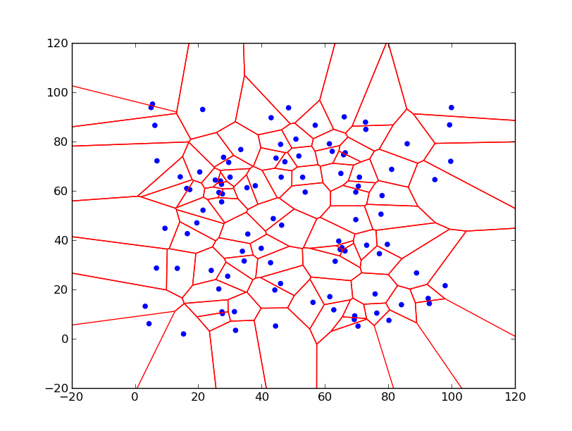
Most common case of Voronoi diagram is known in an Euclidean plane, where we have a set of points (call seeds) then Voronoi diagram splits the plane into areas – called Voronoi cells – around each seed, where inside each area any point is closer to that seed then to any other. Areas are then convex polygons (for Euclidean metric). This definition is best illustrated on the picture below – the Voronoi diagram for 100 random points in range 0-100 – Voronoi cells are marked by red lines, blue points are seeds:
To play with Voronoi diagrams we can use python – recent version of scipy already contains function for calculating Voronoi diagram (see later). But we can use duality of Voronoi diagram to Delaunay triangulation. Both scipy and matplotlib contain functions for Delaunay triangulation. From a given triangulation we can get Voronoi diagram, if we connect centers of circumcircles of each triangle through edges of adjacent triangles. Also there is a pure python implementation of Fortune algorithm available on web here.
Below is the code for calculation Voronoi diagram using Delaunay triangulation function in matplotlib and using numpy for numerical calculations:
#Inspired by code https://github.com/rougier/neural-networks/blob/master/voronoi.py from Nicolas P. Rougier

import sys
import numpy as np
import matplotlib.tri
import matplotlib.pyplot as plt
import time

def circumcircle2(T):
    P1,P2,P3=T[:,0], T[:,1], T[:,2]
    b = P2 - P1
    c = P3 - P1
    d=2*(b[:,0]*c[:,1]-b[:,1]*c[:,0])
    center_x=(c[:,1]*(np.square(b[:,0])+np.square(b[:,1]))- b[:,1]*(np.square(c[:,0])+np.square(c[:,1])))/d + P1[:,0]
    center_y=(b[:,0]*(np.square(c[:,0])+np.square(c[:,1]))- c[:,0]*(np.square(b[:,0])+np.square(b[:,1])))/d + P1[:,1]
    return np.array((center_x, center_y)).T

def check_outside(point, bbox):
    point=np.round(point, 4)
    return point[0]<bbox[0] or point[0]>bbox[2] or point[1]< bbox[1] or point[1]>bbox[3]

def move_point(start, end, bbox):
    vector=end-start
    c=calc_shift(start, vector, bbox)
    if c>0 and c<1:
        start=start+c*vector
        return start

def calc_shift(point, vector, bbox):
    c=sys.float_info.max
    for l,m in enumerate(bbox):
        a=(float(m)-point[l%2])/vector[l%2]
        if  a>0 and  not check_outside(point+a*vector, bbox):
            if abs(a)<abs(c):
                c=a
    return c if c<sys.float_info.max else None

def voronoi2(P, bbox=None):
    if not isinstance(P, np.ndarray):
        P=np.array(P)
    if not bbox:
        xmin=P[:,0].min()
        xmax=P[:,0].max()
        ymin=P[:,1].min()
        ymax=P[:,1].max()
        xrange=(xmax-xmin) * 0.3333333
        yrange=(ymax-ymin) * 0.3333333
        bbox=(xmin-xrange, ymin-yrange, xmax+xrange, ymax+yrange)
    bbox=np.round(bbox,4)

    D = matplotlib.tri.Triangulation(P[:,0],P[:,1])
    T = D.triangles
    n = T.shape[0]
    C = circumcircle2(P[T])

    segments = []
    for i in range(n):
        for j in range(3):
            k = D.neighbors[i][j]
            if k != -1:
                #cut segment to part in bbox
                start,end=C[i], C[k]
                if check_outside(start, bbox):
                    start=move_point(start,end, bbox)
                    if  start is None:
                        continue
                if check_outside(end, bbox):
                    end=move_point(end,start, bbox)
                    if  end is None:
                        continue
                segments.append( [start, end] )
            else:
                #ignore center outside of bbox
                if check_outside(C[i], bbox) :
                    continue
                first, second, third=P[T[i,j]], P[T[i,(j+1)%3]], P[T[i,(j+2)%3]]
                edge=np.array([first, second])
                vector=np.array([[0,1], [-1,0]]).dot(edge[1]-edge[0])
                line=lambda p: (p[0]-first[0])*(second[1]-first[1])/(second[0]-first[0])  -p[1] + first[1]
                orientation=np.sign(line(third))*np.sign( line(first+vector))
                if orientation>0:
                    vector=-orientation*vector
                c=calc_shift(C[i], vector, bbox)
                if c is not None:
                    segments.append([C[i],C[i]+c*vector])
    return segments

if __name__=='__main__':
    points=np.random.rand(100,2)*100
    lines=voronoi2(points, (-20,-20, 120, 120))
    plt.scatter(points[:,0], points[:,1], color="blue")
    lines = matplotlib.collections.LineCollection(lines, color='red')
    plt.gca().add_collection(lines)
    plt.axis((-20,120, -20,120))
    plt.show()
I was inspired by code mentioned on first line comment, I refactor it to leverage numpy matrix computations and also added feature to limit diagram to a bounding box.
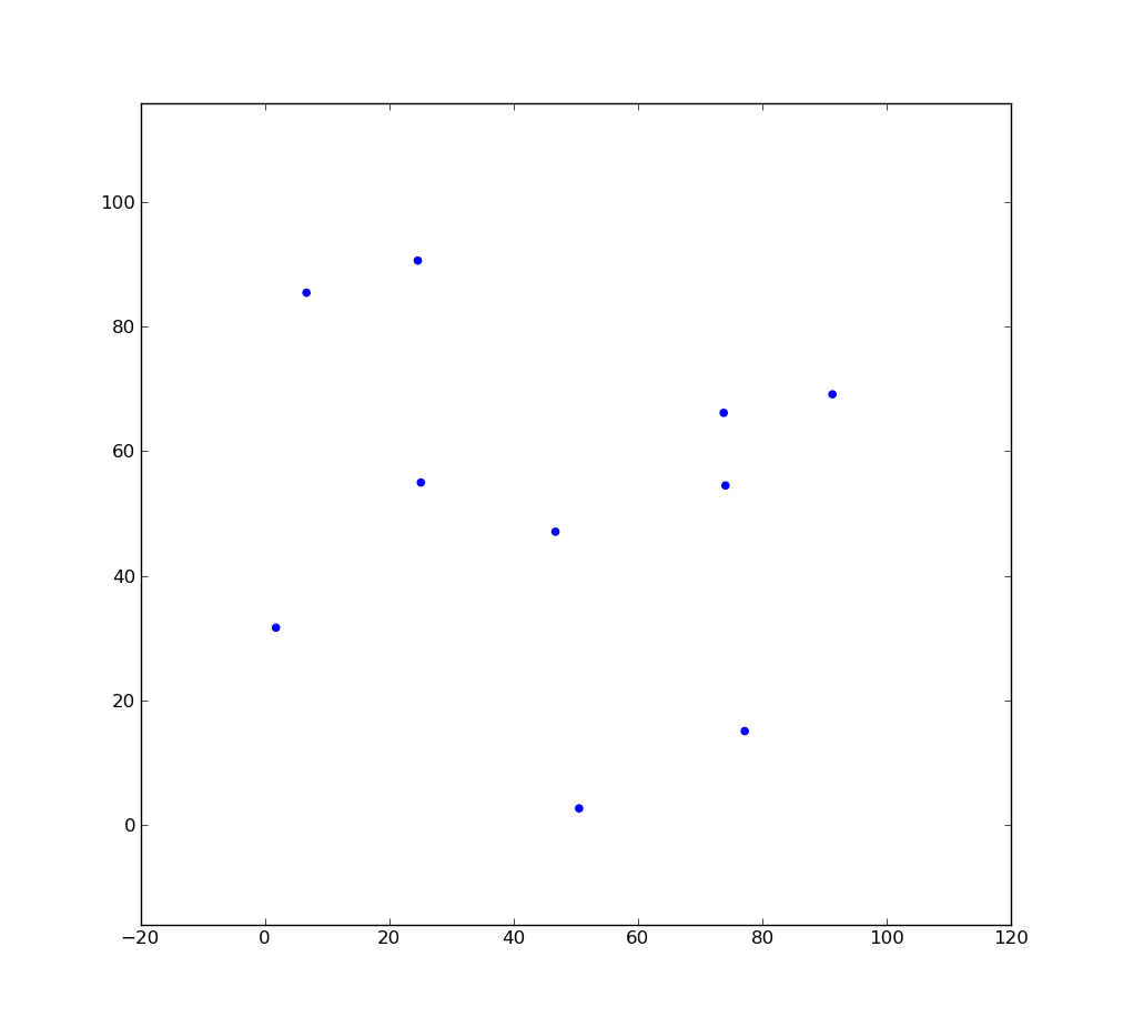
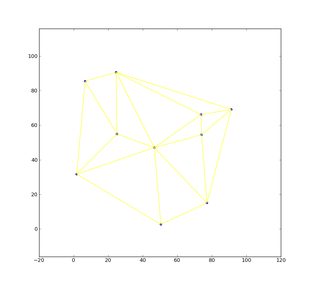
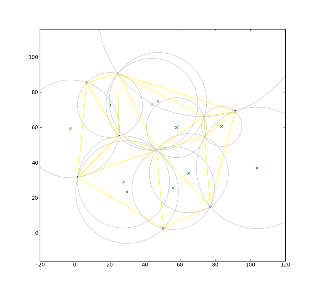
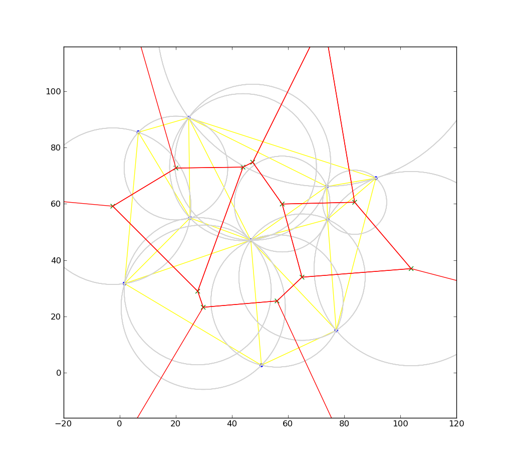
Pictures below illustrateshow Voronoi diagram is created from triangulation – we have a set of seed points (blue), then Delaunay triangulation is calculated (yellow lines), for each triangle we calculate circumcircle – center of circle is green cross and circle itself is grey. Finally we connect circle centers (red lines) and for border triangles we create line from the circumcircle center in direction perpendicular to the outer triangle edge and line extends to infinity ( to bounding box boundary in our case).
As already said there is also function scipy.spatial.Voronoi, which returns directly vertices and edges of Voronoi diagram. Generally this function is faster then our example above (app. 2 – 3 times) – below is code that also calculates missing edges (leading to infinity) and limits picture to a bounding box ( similar to previous example):
import sys
import numpy as np

def check_outside(point, bbox):
    point=np.round(point, 4)
    return point[0]<bbox[0] or point[0]>bbox[2] or point[1]< bbox[1] or point[1]>bbox[3]

def move_point(start, end, bbox):
    vector=end-start
    c=calc_shift(start, vector, bbox)
    if c>0 and c<1:
        start=start+c*vector
        return start

def calc_shift(point, vector, bbox):
    c=sys.float_info.max
    for l,m in enumerate(bbox):
        a=(float(m)-point[l%2])/vector[l%2]
        if  a>0 and  not check_outside(point+a*vector, bbox):
            if abs(a)<abs(c):
                c=a
    return c if c<sys.float_info.max else None

from scipy.spatial import Voronoi
def voronoi3(P, bbox=None):
    P=np.asarray(P)
    if not bbox:
        xmin=P[:,0].min()
        xmax=P[:,0].max()
        ymin=P[:,1].min()
        ymax=P[:,1].max()
        xrange=(xmax-xmin) * 0.3333333
        yrange=(ymax-ymin) * 0.3333333
        bbox=(xmin-xrange, ymin-yrange, xmax+xrange, ymax+yrange)
    bbox=np.round(bbox,4)
    vor=Voronoi(P)
    center = vor.points.mean(axis=0)
    vs=vor.vertices
    segments=[]
    for i,(istart,iend) in enumerate(vor.ridge_vertices):
        if istart<0 or iend<=0:
            start=vs[istart] if istart>=0 else vs[iend]
            if check_outside(start, bbox) :
                    continue
            first,second = vor.ridge_points[i]
            first,second = vor.points[first], vor.points[second]
            edge= second - first
            vector=np.array([-edge[1], edge[0]])
            midpoint= (second+first)/2
            orientation=np.sign(np.dot(midpoint-center, vector))
            vector=orientation*vector
            c=calc_shift(start, vector, bbox)
            if c is not None:
                segments.append([start,start+c*vector])
        else:
            start,end=vs[istart], vs[iend]
            if check_outside(start, bbox):
                start=move_point(start,end, bbox)
                if  start is None:
                    continue
            if check_outside(end, bbox):
                end=move_point(end,start, bbox)
                if  end is None:
                    continue
            segments.append( [start, end] )


    return segments
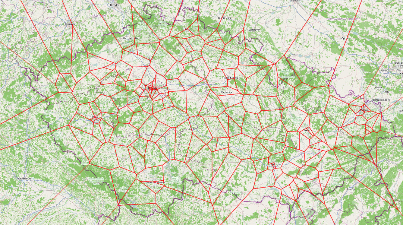
Voronoi diagrams have many different application , some of them in geography – for instance below is a map of Czech Republic, overlayed with Voronoi diagram, where seeds are breweries in that country.
One thought on “Voronoi Diagrams”